Collecting seaborn
  Downloading seaborn-0.13.2-py3-none-any.whl.metadata (5.4 kB)
Requirement already satisfied: numpy!=1.24.0,>=1.20 in c:\users\hp\miniconda3\envs\py312\lib\site-packages (from seaborn) (2.3.1)
Requirement already satisfied: pandas>=1.2 in c:\users\hp\miniconda3\envs\py312\lib\site-packages (from seaborn) (2.3.0)
Requirement already satisfied: matplotlib!=3.6.1,>=3.4 in c:\users\hp\miniconda3\envs\py312\lib\site-packages (from seaborn) (3.10.3)
Requirement already satisfied: contourpy>=1.0.1 in c:\users\hp\miniconda3\envs\py312\lib\site-packages (from matplotlib!=3.6.1,>=3.4->seaborn) (1.3.2)
Requirement already satisfied: cycler>=0.10 in c:\users\hp\miniconda3\envs\py312\lib\site-packages (from matplotlib!=3.6.1,>=3.4->seaborn) (0.12.1)
Requirement already satisfied: fonttools>=4.22.0 in c:\users\hp\miniconda3\envs\py312\lib\site-packages (from matplotlib!=3.6.1,>=3.4->seaborn) (4.58.4)
Requirement already satisfied: kiwisolver>=1.3.1 in c:\users\hp\miniconda3\envs\py312\lib\site-packages (from matplotlib!=3.6.1,>=3.4->seaborn) (1.4.8)
Requirement already satisfied: packaging>=20.0 in c:\users\hp\miniconda3\envs\py312\lib\site-packages (from matplotlib!=3.6.1,>=3.4->seaborn) (24.2)
Requirement already satisfied: pillow>=8 in c:\users\hp\miniconda3\envs\py312\lib\site-packages (from matplotlib!=3.6.1,>=3.4->seaborn) (11.2.1)
Requirement already satisfied: pyparsing>=2.3.1 in c:\users\hp\miniconda3\envs\py312\lib\site-packages (from matplotlib!=3.6.1,>=3.4->seaborn) (3.2.3)
Requirement already satisfied: python-dateutil>=2.7 in c:\users\hp\miniconda3\envs\py312\lib\site-packages (from matplotlib!=3.6.1,>=3.4->seaborn) (2.9.0.post0)
Requirement already satisfied: pytz>=2020.1 in c:\users\hp\miniconda3\envs\py312\lib\site-packages (from pandas>=1.2->seaborn) (2025.2)
Requirement already satisfied: tzdata>=2022.7 in c:\users\hp\miniconda3\envs\py312\lib\site-packages (from pandas>=1.2->seaborn) (2025.2)
Requirement already satisfied: six>=1.5 in c:\users\hp\miniconda3\envs\py312\lib\site-packages (from python-dateutil>=2.7->matplotlib!=3.6.1,>=3.4->seaborn) (1.17.0)
Downloading seaborn-0.13.2-py3-none-any.whl (294 kB)
Installing collected packages: seaborn
Successfully installed seaborn-0.13.2
Note: you may need to restart the kernel to use updated packages.
import pandas as pd
import numpy as np
import matplotlib.pyplot as plt
import seaborn as sns

# Enable inline plotting
%matplotlib inline
data = {
    "Name": ["Alice", "Bob", "Charlie", "David", "Eva", "Frank", "Grace", "Henry"],
    "Age": [25, 30, np.nan, 45, 28, 33, 38, np.nan],
    "Salary": [50000, 60000, 55000, 65000, np.nan, 70000, 62000, 58000],
    "Department": ["HR", "Finance", "IT", "Finance", "HR", "IT", "IT", "HR"]
}
df = pd.DataFrame(data)
df
|
Name |
Age |
Salary |
Department |
| 0 |
Alice |
25.0 |
50000.0 |
HR |
| 1 |
Bob |
30.0 |
60000.0 |
Finance |
| 2 |
Charlie |
NaN |
55000.0 |
IT |
| 3 |
David |
45.0 |
65000.0 |
Finance |
| 4 |
Eva |
28.0 |
NaN |
HR |
| 5 |
Frank |
33.0 |
70000.0 |
IT |
| 6 |
Grace |
38.0 |
62000.0 |
IT |
| 7 |
Henry |
NaN |
58000.0 |
HR |
<class 'pandas.core.frame.DataFrame'>
RangeIndex: 8 entries, 0 to 7
Data columns (total 4 columns):
 #   Column      Non-Null Count  Dtype
---  ------      --------------  -----
 0   Name        8 non-null      object
 1   Age         6 non-null      float64
 2   Salary      7 non-null      float64
 3   Department  8 non-null      object
dtypes: float64(2), object(2)
memory usage: 388.0+ bytes
Name          0
Age           2
Salary        1
Department    0
dtype: int64
df['Age'] = df['Age'].fillna(df['Age'].median())
df
|
Name |
Age |
Salary |
Department |
| 0 |
Alice |
25.0 |
50000.0 |
HR |
| 1 |
Bob |
30.0 |
60000.0 |
Finance |
| 2 |
Charlie |
31.5 |
55000.0 |
IT |
| 3 |
David |
45.0 |
65000.0 |
Finance |
| 4 |
Eva |
28.0 |
NaN |
HR |
| 5 |
Frank |
33.0 |
70000.0 |
IT |
| 6 |
Grace |
38.0 |
62000.0 |
IT |
| 7 |
Henry |
31.5 |
58000.0 |
HR |
df['Salary'] = df['Salary'].fillna(df['Salary'].mean())
df
|
Name |
Age |
Salary |
Department |
| 0 |
Alice |
25.0 |
50000.0 |
HR |
| 1 |
Bob |
30.0 |
60000.0 |
Finance |
| 2 |
Charlie |
31.5 |
55000.0 |
IT |
| 3 |
David |
45.0 |
65000.0 |
Finance |
| 4 |
Eva |
28.0 |
60000.0 |
HR |
| 5 |
Frank |
33.0 |
70000.0 |
IT |
| 6 |
Grace |
38.0 |
62000.0 |
IT |
| 7 |
Henry |
31.5 |
58000.0 |
HR |
|
Age |
Salary |
| count |
8.00000 |
8.000000 |
| mean |
32.75000 |
60000.000000 |
| std |
6.22208 |
6071.008389 |
| min |
25.00000 |
50000.000000 |
| 25% |
29.50000 |
57250.000000 |
| 50% |
31.50000 |
60000.000000 |
| 75% |
34.25000 |
62750.000000 |
| max |
45.00000 |
70000.000000 |
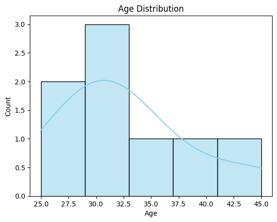
sns.histplot(df['Age'], kde=True, bins=5, color='skyblue')
plt.title("Age Distribution")
plt.xlabel("Age")
plt.ylabel("Count")
plt.show()
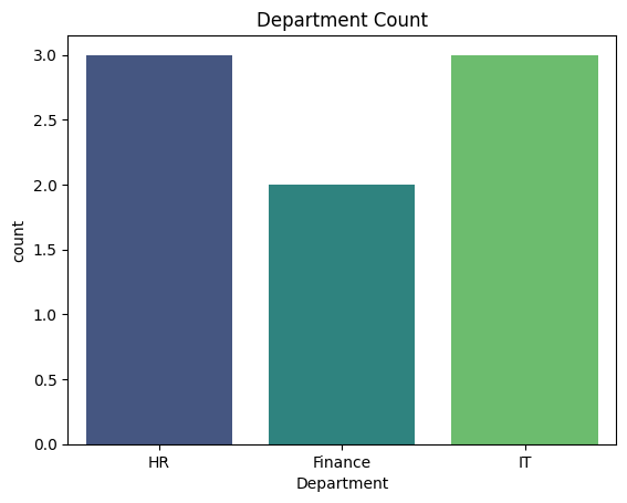
sns.countplot(x="Department", data=df, palette="viridis")
plt.title("Department Count")
plt.show()
C:\Users\HP\AppData\Local\Temp\ipykernel_1960\1748937494.py:1: FutureWarning:

Passing `palette` without assigning `hue` is deprecated and will be removed in v0.14.0. Assign the `x` variable to `hue` and set `legend=False` for the same effect.

  sns.countplot(x="Department", data=df, palette="viridis")
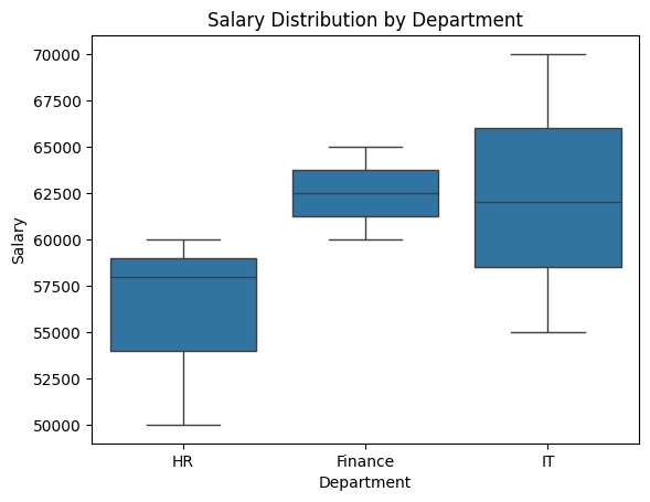
sns.boxplot(x="Department", y="Salary", data=df)
plt.title("Salary Distribution by Department")
plt.show()
df['Experience'] = [2, 5, 3, 10, 4, 8, 6, 7]
df
|
Name |
Age |
Salary |
Department |
Experience |
| 0 |
Alice |
25.0 |
50000.0 |
HR |
2 |
| 1 |
Bob |
30.0 |
60000.0 |
Finance |
5 |
| 2 |
Charlie |
31.5 |
55000.0 |
IT |
3 |
| 3 |
David |
45.0 |
65000.0 |
Finance |
10 |
| 4 |
Eva |
28.0 |
60000.0 |
HR |
4 |
| 5 |
Frank |
33.0 |
70000.0 |
IT |
8 |
| 6 |
Grace |
38.0 |
62000.0 |
IT |
6 |
| 7 |
Henry |
31.5 |
58000.0 |
HR |
7 |
df.corr(numeric_only=True)
|
Age |
Salary |
Experience |
| Age |
1.000000 |
0.606989 |
0.819292 |
| Salary |
0.606989 |
1.000000 |
0.819845 |
| Experience |
0.819292 |
0.819845 |
1.000000 |
df.corr(numeric_only=True)
|
Age |
Salary |
Experience |
| Age |
1.000000 |
0.606989 |
0.819292 |
| Salary |
0.606989 |
1.000000 |
0.819845 |
| Experience |
0.819292 |
0.819845 |
1.000000 |
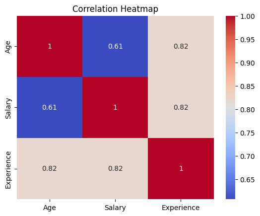
sns.heatmap(df.corr(numeric_only=True), annot=True, cmap='coolwarm')
plt.title("Correlation Heatmap")
plt.show()
|
Name |
Age |
Salary |
Department |
Experience |
| 3 |
David |
45.0 |
65000.0 |
Finance |
10 |
| 5 |
Frank |
33.0 |
70000.0 |
IT |
8 |
| 6 |
Grace |
38.0 |
62000.0 |
IT |
6 |
df.groupby('Department')['Salary'].mean()
Department
Finance    62500.000000
HR         56000.000000
IT         62333.333333
Name: Salary, dtype: float64
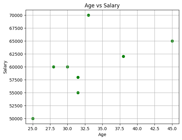
plt.scatter(df['Age'], df['Salary'], color='green')
plt.xlabel('Age')
plt.ylabel('Salary')
plt.title('Age vs Salary')
plt.grid(True)
plt.show()
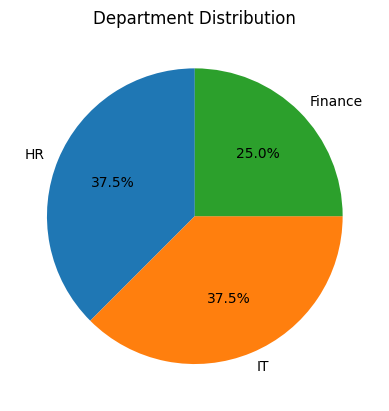
df['Department'].value_counts().plot.pie(autopct='%1.1f%%', startangle=90)
plt.title('Department Distribution')
plt.ylabel('')
plt.show()
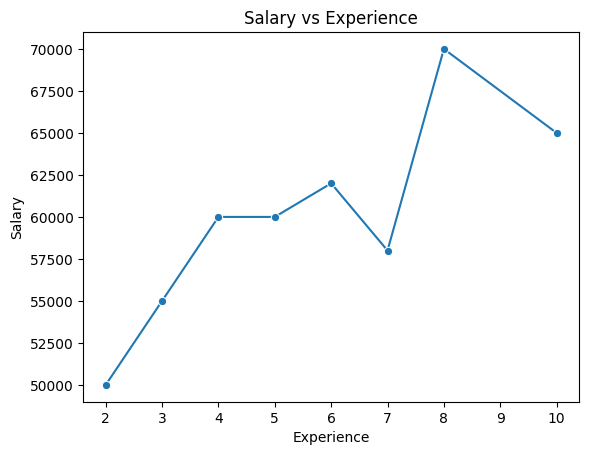
sns.lineplot(x='Experience', y='Salary', data=df, marker='o')
plt.title("Salary vs Experience")
plt.show()
df['Bonus'] = df['Salary'] * 0.1
df
|
Name |
Age |
Salary |
Department |
Experience |
Bonus |
| 0 |
Alice |
25.0 |
50000.0 |
HR |
2 |
5000.0 |
| 1 |
Bob |
30.0 |
60000.0 |
Finance |
5 |
6000.0 |
| 2 |
Charlie |
31.5 |
55000.0 |
IT |
3 |
5500.0 |
| 3 |
David |
45.0 |
65000.0 |
Finance |
10 |
6500.0 |
| 4 |
Eva |
28.0 |
60000.0 |
HR |
4 |
6000.0 |
| 5 |
Frank |
33.0 |
70000.0 |
IT |
8 |
7000.0 |
| 6 |
Grace |
38.0 |
62000.0 |
IT |
6 |
6200.0 |
| 7 |
Henry |
31.5 |
58000.0 |
HR |
7 |
5800.0 |
|
Name |
Age |
Salary |
Department |
Experience |
Bonus |
| 0 |
Alice |
25.0 |
50000.0 |
HR |
2 |
5000.0 |
| 1 |
Bob |
30.0 |
60000.0 |
Finance |
5 |
6000.0 |
| 2 |
Charlie |
31.5 |
55000.0 |
IT |
3 |
5500.0 |
| 3 |
David |
45.0 |
65000.0 |
Finance |
10 |
6500.0 |
| 4 |
Eva |
28.0 |
60000.0 |
HR |
4 |
6000.0 |
df.to_csv("cleaned_employee_data.csv", index=False)
print("Saved to cleaned_employee_data.csv")
Saved to cleaned_employee_data.csv
Score: 20