Iris
Mon 30 June 2025
import pandas as pd
import seaborn as sns
import matplotlib.pyplot as plt
from sklearn.datasets import load_iris
iris = load_iris()
df = pd.DataFrame(iris.data, columns=iris.feature_names)
df['species'] = iris.target
df['species'] = df['species'].map(dict(enumerate(iris.target_names)))
df.head()
| sepal length (cm) | sepal width (cm) | petal length (cm) | petal width (cm) | species | |
|---|---|---|---|---|---|
| 0 | 5.1 | 3.5 | 1.4 | 0.2 | setosa |
| 1 | 4.9 | 3.0 | 1.4 | 0.2 | setosa |
| 2 | 4.7 | 3.2 | 1.3 | 0.2 | setosa |
| 3 | 4.6 | 3.1 | 1.5 | 0.2 | setosa |
| 4 | 5.0 | 3.6 | 1.4 | 0.2 | setosa |
df.isnull().sum()
sepal length (cm)    0
sepal width (cm)     0
petal length (cm)    0
petal width (cm)     0
species              0
dtype: int64
df.describe()
| sepal length (cm) | sepal width (cm) | petal length (cm) | petal width (cm) | |
|---|---|---|---|---|
| count | 150.000000 | 150.000000 | 150.000000 | 150.000000 |
| mean | 5.843333 | 3.057333 | 3.758000 | 1.199333 |
| std | 0.828066 | 0.435866 | 1.765298 | 0.762238 |
| min | 4.300000 | 2.000000 | 1.000000 | 0.100000 |
| 25% | 5.100000 | 2.800000 | 1.600000 | 0.300000 |
| 50% | 5.800000 | 3.000000 | 4.350000 | 1.300000 |
| 75% | 6.400000 | 3.300000 | 5.100000 | 1.800000 |
| max | 7.900000 | 4.400000 | 6.900000 | 2.500000 |
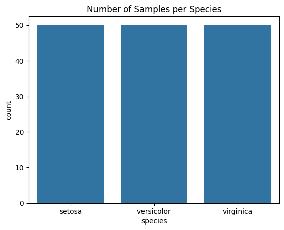
sns.countplot(x='species', data=df)
plt.title("Number of Samples per Species")
plt.show()
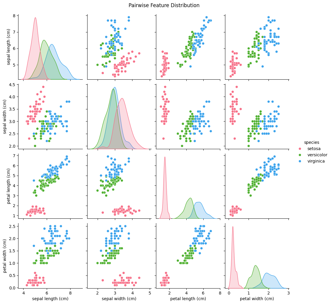
sns.pairplot(df, hue="species", palette="husl")
plt.suptitle("Pairwise Feature Distribution", y=1.02)
plt.show()
corr = df.drop('species', axis=1).corr()
corr
| sepal length (cm) | sepal width (cm) | petal length (cm) | petal width (cm) | |
|---|---|---|---|---|
| sepal length (cm) | 1.000000 | -0.117570 | 0.871754 | 0.817941 |
| sepal width (cm) | -0.117570 | 1.000000 | -0.428440 | -0.366126 |
| petal length (cm) | 0.871754 | -0.428440 | 1.000000 | 0.962865 |
| petal width (cm) | 0.817941 | -0.366126 | 0.962865 | 1.000000 |
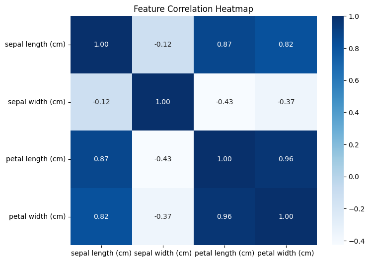
plt.figure(figsize=(8,6))
sns.heatmap(corr, annot=True, cmap='Blues', fmt=".2f")
plt.title("Feature Correlation Heatmap")
plt.show()
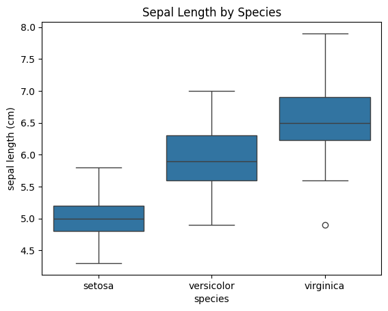
sns.boxplot(x="species", y="sepal length (cm)", data=df)
plt.title("Sepal Length by Species")
plt.show()
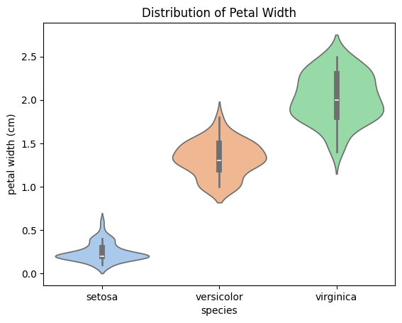
sns.violinplot(x="species", y="petal width (cm)", data=df, palette="pastel")
plt.title("Distribution of Petal Width")
plt.show()
C:\Users\HP\AppData\Local\Temp\ipykernel_19564\2798115140.py:1: FutureWarning:

Passing `palette` without assigning `hue` is deprecated and will be removed in v0.14.0. Assign the `x` variable to `hue` and set `legend=False` for the same effect.

  sns.violinplot(x="species", y="petal width (cm)", data=df, palette="pastel")
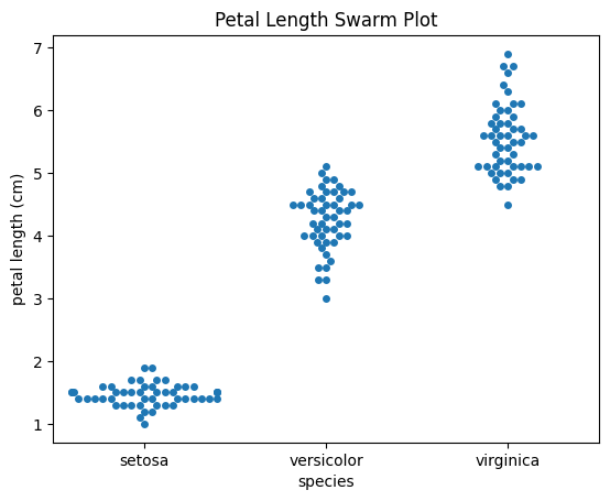
sns.swarmplot(x="species", y="petal length (cm)", data=df)
plt.title("Petal Length Swarm Plot")
plt.show()
C:\Users\HP\miniconda3\envs\py312\Lib\site-packages\seaborn\categorical.py:3399: UserWarning: 12.0% of the points cannot be placed; you may want to decrease the size of the markers or use stripplot.
  warnings.warn(msg, UserWarning)
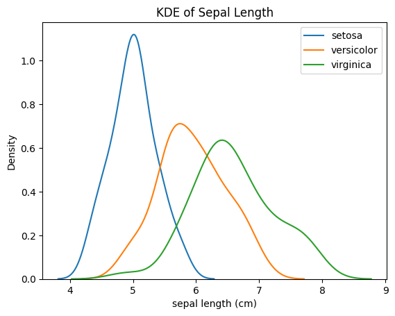
for species in df['species'].unique():
    sns.kdeplot(df[df['species'] == species]['sepal length (cm)'], label=species)
plt.title("KDE of Sepal Length")
plt.legend()
plt.show()
sns.histplot(data=df, x="petal width (cm)", hue="species", kde=True, multiple="stack")
plt.title("Petal Width Histogram by Species")
plt.show()
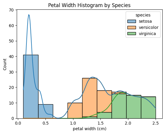
print("Setosa flowers have significantly smaller petals.")
print("Versicolor and Virginica are closer in petal width but differ in sepal length.")
Setosa flowers have significantly smaller petals.
Versicolor and Virginica are closer in petal width but differ in sepal length.
Score: 15
Category: basics