Loan
Mon 30 June 2025
# Block 1: Import libraries
import pandas as pd
import numpy as np
import seaborn as sns
import matplotlib.pyplot as plt
# Block 2: Load the dataset
df = pd.read_csv("https://raw.githubusercontent.com/datasciencedojo/datasets/master/titanic.csv")
df = df.rename(columns={"Sex": "Gender", "Age": "ApplicantIncome", "Fare": "LoanAmount"})
df = df[["Gender", "ApplicantIncome", "LoanAmount", "Pclass", "Embarked", "Survived"]]
df.head()
| Gender | ApplicantIncome | LoanAmount | Pclass | Embarked | Survived | |
|---|---|---|---|---|---|---|
| 0 | male | 22.0 | 7.2500 | 3 | S | 0 |
| 1 | female | 38.0 | 71.2833 | 1 | C | 1 |
| 2 | female | 26.0 | 7.9250 | 3 | S | 1 |
| 3 | female | 35.0 | 53.1000 | 1 | S | 1 |
| 4 | male | 35.0 | 8.0500 | 3 | S | 0 |
# Block 3: Check data types and missing values
df.info()
<class 'pandas.core.frame.DataFrame'>
RangeIndex: 891 entries, 0 to 890
Data columns (total 6 columns):
 #   Column           Non-Null Count  Dtype
---  ------           --------------  -----
 0   Gender           891 non-null    object
 1   ApplicantIncome  714 non-null    float64
 2   LoanAmount       891 non-null    float64
 3   Pclass           891 non-null    int64
 4   Embarked         889 non-null    object
 5   Survived         891 non-null    int64
dtypes: float64(2), int64(2), object(2)
memory usage: 41.9+ KB
# Block 4: Check missing values
df.isnull().sum()
Gender               0
ApplicantIncome    177
LoanAmount           0
Pclass               0
Embarked             2
Survived             0
dtype: int64
# Block 5: Fill missing values
df.loc[:, 'ApplicantIncome'] = df['ApplicantIncome'].fillna(df['ApplicantIncome'].median())
df.loc[:, 'Embarked'] = df['Embarked'].fillna(df['Embarked'].mode()[0])
# Block 6: Convert categorical to numeric
df['Gender'] = df['Gender'].map({'male': 1, 'female': 0})
df['Embarked'] = df['Embarked'].map({'S': 0, 'C': 1, 'Q': 2})
# Block 7: Add artificial label column (1 = eligible, 0 = not eligible)
df['Loan_Approved'] = (df['Survived'] & (df['ApplicantIncome'] > 20) & (df['Pclass'] < 3)).astype(int)
df.drop("Survived", axis=1, inplace=True)
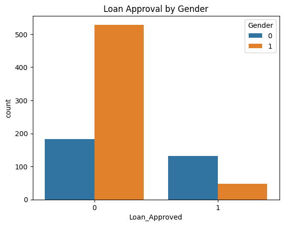
# Block 8: Visualize Loan Approval by Gender
sns.countplot(x='Loan_Approved', hue='Gender', data=df)
plt.title("Loan Approval by Gender")
plt.show()
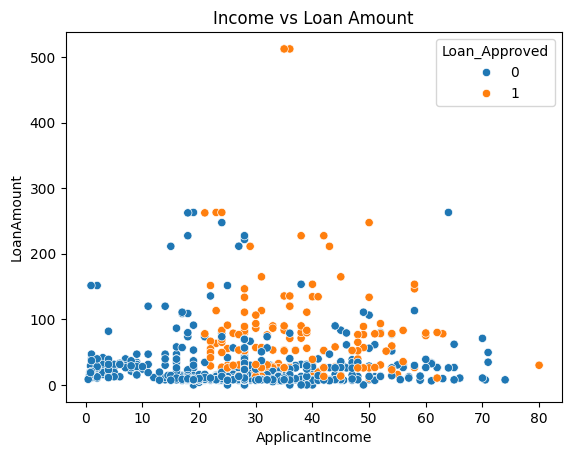
# Block 9: Loan Amount vs Income
sns.scatterplot(x='ApplicantIncome', y='LoanAmount', hue='Loan_Approved', data=df)
plt.title("Income vs Loan Amount")
plt.show()
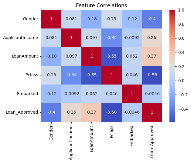
# Block 10: Correlation heatmap
sns.heatmap(df.corr(), annot=True, cmap='coolwarm')
plt.title("Feature Correlations")
plt.show()
# Block 11: Features and Labels
X = df.drop("Loan_Approved", axis=1)
y = df["Loan_Approved"]
# Block 12: Train-test split
from sklearn.model_selection import train_test_split
X_train, X_test, y_train, y_test = train_test_split(X, y, test_size=0.2, random_state=42)
# Block 13: Train Logistic Regression model
from sklearn.linear_model import LogisticRegression
model = LogisticRegression()
model.fit(X_train, y_train)
LogisticRegression()In a Jupyter environment, please rerun this cell to show the HTML representation or trust the notebook.
On GitHub, the HTML representation is unable to render, please try loading this page with nbviewer.org.
Parameters
| penalty | 'l2' | |
| dual | False | |
| tol | 0.0001 | |
| C | 1.0 | |
| fit_intercept | True | |
| intercept_scaling | 1 | |
| class_weight | None | |
| random_state | None | |
| solver | 'lbfgs' | |
| max_iter | 100 | |
| multi_class | 'deprecated' | |
| verbose | 0 | |
| warm_start | False | |
| n_jobs | None | |
| l1_ratio | None |
# Block 14: Predictions and accuracy
from sklearn.metrics import accuracy_score
y_pred = model.predict(X_test)
accuracy_score(y_test, y_pred)
0.8268156424581006
# Block 15: Predict sample data
sample = pd.DataFrame([[1, 50, 200, 1, 0]], columns=X.columns)
model.predict(sample)
array([0])
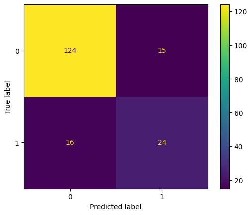
# Block 16: Confusion matrix
from sklearn.metrics import confusion_matrix, ConfusionMatrixDisplay
cm = confusion_matrix(y_test, y_pred)
ConfusionMatrixDisplay(cm).plot()
plt.show()
Score: 15
Category: basics