Sales
Mon 30 June 2025
import pandas as pd
import matplotlib.pyplot as plt
import seaborn as sns

sns.set(style="whitegrid")
data = {
    "OrderID": [1001, 1002, 1003, 1004, 1005, 1006],
    "Product": ["Laptop", "Mouse", "Keyboard", "Monitor", "Laptop", "Mouse"],
    "Category": ["Electronics", "Accessories", "Accessories", "Electronics", "Electronics", "Accessories"],
    "Price": [70000, 500, 1500, 12000, 72000, 550],
    "Quantity": [1, 2, 1, 2, 1, 3],
    "Date": pd.to_datetime(["2023-01-10", "2023-01-10", "2023-01-11", "2023-01-12", "2023-01-12", "2023-01-13"])
}
df = pd.DataFrame(data)
df
| OrderID | Product | Category | Price | Quantity | Date | |
|---|---|---|---|---|---|---|
| 0 | 1001 | Laptop | Electronics | 70000 | 1 | 2023-01-10 |
| 1 | 1002 | Mouse | Accessories | 500 | 2 | 2023-01-10 |
| 2 | 1003 | Keyboard | Accessories | 1500 | 1 | 2023-01-11 |
| 3 | 1004 | Monitor | Electronics | 12000 | 2 | 2023-01-12 |
| 4 | 1005 | Laptop | Electronics | 72000 | 1 | 2023-01-12 |
| 5 | 1006 | Mouse | Accessories | 550 | 3 | 2023-01-13 |
df["Revenue"] = df["Price"] * df["Quantity"]
df
| OrderID | Product | Category | Price | Quantity | Date | Revenue | |
|---|---|---|---|---|---|---|---|
| 0 | 1001 | Laptop | Electronics | 70000 | 1 | 2023-01-10 | 70000 |
| 1 | 1002 | Mouse | Accessories | 500 | 2 | 2023-01-10 | 1000 |
| 2 | 1003 | Keyboard | Accessories | 1500 | 1 | 2023-01-11 | 1500 |
| 3 | 1004 | Monitor | Electronics | 12000 | 2 | 2023-01-12 | 24000 |
| 4 | 1005 | Laptop | Electronics | 72000 | 1 | 2023-01-12 | 72000 |
| 5 | 1006 | Mouse | Accessories | 550 | 3 | 2023-01-13 | 1650 |
df.describe()
| OrderID | Price | Quantity | Date | Revenue | |
|---|---|---|---|---|---|
| count | 6.000000 | 6.000000 | 6.000000 | 6 | 6.000000 |
| mean | 1003.500000 | 26091.666667 | 1.666667 | 2023-01-11 08:00:00 | 28358.333333 |
| min | 1001.000000 | 500.000000 | 1.000000 | 2023-01-10 00:00:00 | 1000.000000 |
| 25% | 1002.250000 | 787.500000 | 1.000000 | 2023-01-10 06:00:00 | 1537.500000 |
| 50% | 1003.500000 | 6750.000000 | 1.500000 | 2023-01-11 12:00:00 | 12825.000000 |
| 75% | 1004.750000 | 55500.000000 | 2.000000 | 2023-01-12 00:00:00 | 58500.000000 |
| max | 1006.000000 | 72000.000000 | 3.000000 | 2023-01-13 00:00:00 | 72000.000000 |
| std | 1.870829 | 35060.382438 | 0.816497 | NaN | 34178.361820 |
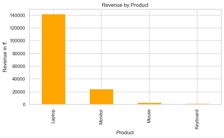
revenue_by_product = df.groupby("Product")["Revenue"].sum().sort_values(ascending=False)
revenue_by_product
Product
Laptop      142000
Monitor      24000
Mouse         2650
Keyboard      1500
Name: Revenue, dtype: int64
revenue_by_product.plot(kind='bar', color='orange', figsize=(8,4))
plt.title("Revenue by Product")
plt.ylabel("Revenue in ₹")
plt.show()
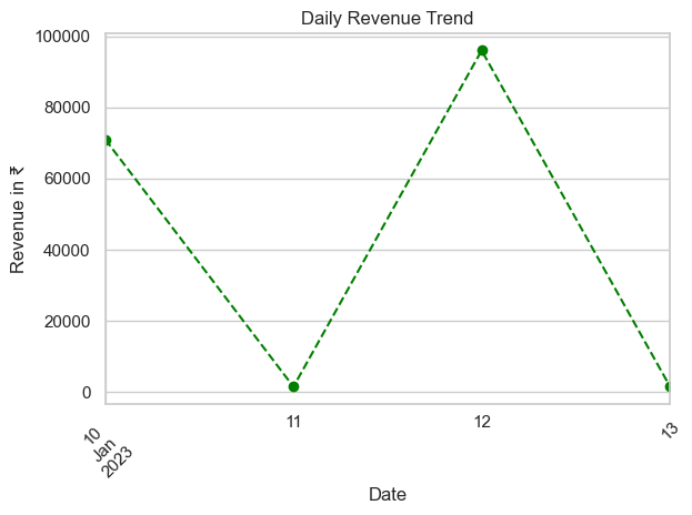
daily_revenue = df.groupby("Date")["Revenue"].sum()
daily_revenue
Date
2023-01-10    71000
2023-01-11     1500
2023-01-12    96000
2023-01-13     1650
Name: Revenue, dtype: int64
daily_revenue.plot(marker='o', linestyle='--', color='green')
plt.title("Daily Revenue Trend")
plt.xlabel("Date")
plt.ylabel("Revenue in ₹")
plt.xticks(rotation=45)
plt.tight_layout()
plt.show()
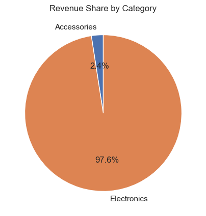
category_revenue = df.groupby("Category")["Revenue"].sum()
category_revenue
Category
Accessories      4150
Electronics    166000
Name: Revenue, dtype: int64
category_revenue.plot.pie(autopct='%1.1f%%', startangle=90, figsize=(5,5))
plt.title("Revenue Share by Category")
plt.ylabel("")
plt.show()
df["Discount"] = [0, 50, 0, 1000, 0, 30]  # Simulate discounts
df["NetRevenue"] = df["Revenue"] - df["Discount"]
df
| OrderID | Product | Category | Price | Quantity | Date | Revenue | Discount | NetRevenue | |
|---|---|---|---|---|---|---|---|---|---|
| 0 | 1001 | Laptop | Electronics | 70000 | 1 | 2023-01-10 | 70000 | 0 | 70000 |
| 1 | 1002 | Mouse | Accessories | 500 | 2 | 2023-01-10 | 1000 | 50 | 950 |
| 2 | 1003 | Keyboard | Accessories | 1500 | 1 | 2023-01-11 | 1500 | 0 | 1500 |
| 3 | 1004 | Monitor | Electronics | 12000 | 2 | 2023-01-12 | 24000 | 1000 | 23000 |
| 4 | 1005 | Laptop | Electronics | 72000 | 1 | 2023-01-12 | 72000 | 0 | 72000 |
| 5 | 1006 | Mouse | Accessories | 550 | 3 | 2023-01-13 | 1650 | 30 | 1620 |
df[["Revenue", "NetRevenue"]].sum()
Revenue       170150
NetRevenue    169070
dtype: int64
df.loc[df["Revenue"].idxmax()]
OrderID                      1005
Product                    Laptop
Category              Electronics
Price                       72000
Quantity                        1
Date          2023-01-12 00:00:00
Revenue                     72000
Discount                        0
NetRevenue                  72000
Name: 4, dtype: object
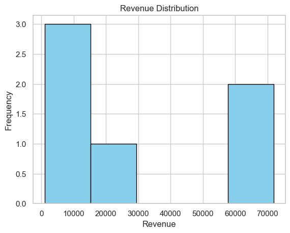
plt.hist(df["Revenue"], bins=5, color="skyblue", edgecolor="black")
plt.title("Revenue Distribution")
plt.xlabel("Revenue")
plt.ylabel("Frequency")
plt.show()
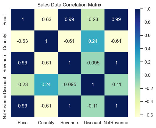
correlation = df[["Price", "Quantity", "Revenue", "Discount", "NetRevenue"]].corr()
sns.heatmap(correlation, annot=True, cmap="YlGnBu")
plt.title("Sales Data Correlation Matrix")
plt.show()
summary = df.groupby("Product")[["Quantity", "Revenue", "Discount", "NetRevenue"]].sum()
summary
| Quantity | Revenue | Discount | NetRevenue | |
|---|---|---|---|---|
| Product | ||||
| Keyboard | 1 | 1500 | 0 | 1500 |
| Laptop | 2 | 142000 | 0 | 142000 |
| Monitor | 2 | 24000 | 1000 | 23000 |
| Mouse | 5 | 2650 | 80 | 2570 |
Score: 15
Category: basics