Stock
Mon 30 June 2025
# Block 1: Install required packages (if not already installed)
!pip install yfinance matplotlib --quiet
# Block 2: Import necessary libraries
import yfinance as yf
import matplotlib.pyplot as plt
import pandas as pd
# Block 3: Set display options for better visualization
pd.set_option("display.max_rows", 10)
pd.set_option("display.float_format", "{:.2f}".format)
# Block 4: Download historical stock data for Apple (AAPL)
stock = yf.Ticker("AAPL")
df = stock.history(period="1y")
df.head()
| Open | High | Low | Close | Volume | Dividends | Stock Splits | |
|---|---|---|---|---|---|---|---|
| Date | |||||||
| 2024-06-28 00:00:00-04:00 | 214.77 | 215.06 | 209.32 | 209.64 | 82542700 | 0.00 | 0.00 |
| 2024-07-01 00:00:00-04:00 | 211.10 | 216.50 | 210.93 | 215.74 | 60402900 | 0.00 | 0.00 |
| 2024-07-02 00:00:00-04:00 | 215.14 | 219.35 | 214.10 | 219.24 | 58046200 | 0.00 | 0.00 |
| 2024-07-03 00:00:00-04:00 | 218.98 | 220.52 | 218.01 | 220.52 | 37369800 | 0.00 | 0.00 |
| 2024-07-05 00:00:00-04:00 | 220.62 | 225.40 | 220.62 | 225.29 | 60412400 | 0.00 | 0.00 |
# Block 5: Basic Information
print("Company Info:")
stock.info['longBusinessSummary'][:300] + "..."
Company Info:


'Apple Inc. designs, manufactures, and markets smartphones, personal computers, tablets, wearables, and accessories worldwide. The company offers iPhone, a line of smartphones; Mac, a line of personal computers; iPad, a line of multi-purpose tablets; and wearables, home, and accessories comprising Ai...'
# Block 6: Describe the dataset
df.describe()
| Open | High | Low | Close | Volume | Dividends | Stock Splits | |
|---|---|---|---|---|---|---|---|
| count | 250.00 | 250.00 | 250.00 | 250.00 | 250.00 | 250.00 | 250.00 |
| mean | 222.36 | 224.92 | 220.02 | 222.67 | 53516737.60 | 0.00 | 0.00 |
| std | 15.69 | 15.12 | 15.96 | 15.61 | 27343853.63 | 0.03 | 0.00 |
| min | 171.72 | 190.09 | 168.99 | 172.19 | 23234700.00 | 0.00 | 0.00 |
| 25% | 211.19 | 214.02 | 209.38 | 212.35 | 39510475.00 | 0.00 | 0.00 |
| 50% | 224.17 | 226.07 | 222.23 | 224.21 | 46906700.00 | 0.00 | 0.00 |
| 75% | 232.45 | 234.26 | 229.18 | 232.52 | 58825975.00 | 0.00 | 0.00 |
| max | 257.57 | 259.47 | 257.01 | 258.40 | 318679900.00 | 0.26 | 0.00 |
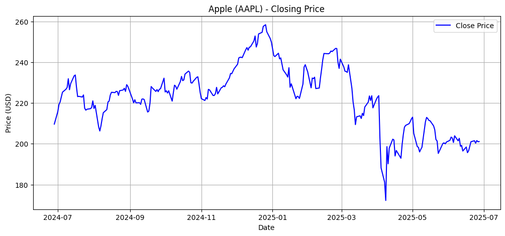
# Block 7: Plot closing price
plt.figure(figsize=(12, 5))
plt.plot(df['Close'], label="Close Price", color='blue')
plt.title("Apple (AAPL) - Closing Price")
plt.xlabel("Date")
plt.ylabel("Price (USD)")
plt.legend()
plt.grid(True)
plt.show()
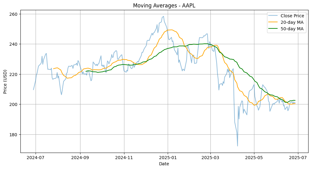
# Block 8: Calculate Moving Averages
df['MA20'] = df['Close'].rolling(window=20).mean()
df['MA50'] = df['Close'].rolling(window=50).mean()
df[['Close', 'MA20', 'MA50']].tail()
| Close | MA20 | MA50 | |
|---|---|---|---|
| Date | |||
| 2025-06-23 00:00:00-04:00 | 201.50 | 200.04 | 202.30 |
| 2025-06-24 00:00:00-04:00 | 200.30 | 200.29 | 202.50 |
| 2025-06-25 00:00:00-04:00 | 201.56 | 200.36 | 202.57 |
| 2025-06-26 00:00:00-04:00 | 201.00 | 200.38 | 202.55 |
| 2025-06-27 00:00:00-04:00 | 201.08 | 200.44 | 202.53 |
# Block 9: Plot Moving Averages
plt.figure(figsize=(12, 6))
plt.plot(df['Close'], label='Close Price', alpha=0.5)
plt.plot(df['MA20'], label='20-day MA', color='orange')
plt.plot(df['MA50'], label='50-day MA', color='green')
plt.title("Moving Averages - AAPL")
plt.xlabel("Date")
plt.ylabel("Price (USD)")
plt.legend()
plt.grid(True)
plt.show()
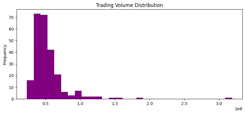
# Block 10: Volume analysis
df['Volume'].plot(kind='hist', bins=30, color='purple', figsize=(10, 4), title='Trading Volume Distribution')
<Axes: title={'center': 'Trading Volume Distribution'}, ylabel='Frequency'>
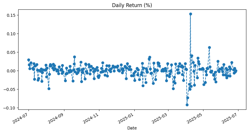
# Block 11: Daily Returns
df['Daily Return'] = df['Close'].pct_change()
df['Daily Return'].dropna().plot(figsize=(10, 5), linestyle='--', marker='o', title="Daily Return (%)")
<Axes: title={'center': 'Daily Return (%)'}, xlabel='Date'>
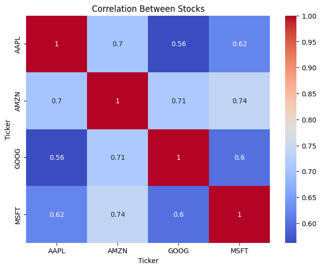
# Block 12: Correlation Matrix (simulate multiple stocks)
tickers = ['AAPL', 'MSFT', 'GOOG', 'AMZN']
df_multi = yf.download(tickers, period="6mo")['Close']
df_multi = df_multi.pct_change().dropna()
correlation = df_multi.corr()
correlation
C:\Users\HP\AppData\Local\Temp\ipykernel_6508\2024470801.py:3: FutureWarning: YF.download() has changed argument auto_adjust default to True
  df_multi = yf.download(tickers, period="6mo")['Close']
[*********************100%***********************]  4 of 4 completed
| Ticker | AAPL | AMZN | GOOG | MSFT |
|---|---|---|---|---|
| Ticker | ||||
| AAPL | 1.00 | 0.70 | 0.56 | 0.62 |
| AMZN | 0.70 | 1.00 | 0.71 | 0.74 |
| GOOG | 0.56 | 0.71 | 1.00 | 0.60 |
| MSFT | 0.62 | 0.74 | 0.60 | 1.00 |
# Block 13: Heatmap of correlation
import seaborn as sns
plt.figure(figsize=(8, 6))
sns.heatmap(correlation, annot=True, cmap="coolwarm")
plt.title("Correlation Between Stocks")
Text(0.5, 1.0, 'Correlation Between Stocks')
# Block 14: Candlestick Chart (optional for advanced visuals)
!pip install plotly
Requirement already satisfied: plotly in c:\users\hp\miniconda3\envs\py312\lib\site-packages (6.2.0)
Requirement already satisfied: narwhals>=1.15.1 in c:\users\hp\miniconda3\envs\py312\lib\site-packages (from plotly) (1.44.0)
Requirement already satisfied: packaging in c:\users\hp\miniconda3\envs\py312\lib\site-packages (from plotly) (24.2)
import plotly.graph_objects as go
fig = go.Figure(data=[go.Candlestick(x=df.index,
                open=df['Open'],
                high=df['High'],
                low=df['Low'],
                close=df['Close'])])
fig.update_layout(title='Candlestick Chart - AAPL', xaxis_rangeslider_visible=False)
fig.show()
# Block 15: Highest closing price
highest = df['Close'].max()
print(f"Highest Closing Price in the Last 1 Year: ${highest:.2f}")
Highest Closing Price in the Last 1 Year: $258.40
# Block 16: Lowest closing price
lowest = df['Close'].min()
print(f"Lowest Closing Price in the Last 1 Year: ${lowest:.2f}")
Lowest Closing Price in the Last 1 Year: $172.19
# Block 17: Save processed data to CSV
df.to_csv("AAPL_Processed.csv")
print("Saved to AAPL_Processed.csv")
Saved to AAPL_Processed.csv
# Block 18: Display final data sample
df.tail()
| Open | High | Low | Close | Volume | Dividends | Stock Splits | MA20 | MA50 | Daily Return | |
|---|---|---|---|---|---|---|---|---|---|---|
| Date | ||||||||||
| 2025-06-23 00:00:00-04:00 | 201.63 | 202.30 | 198.96 | 201.50 | 55814300 | 0.00 | 0.00 | 200.04 | 202.30 | 0.00 |
| 2025-06-24 00:00:00-04:00 | 202.59 | 203.44 | 200.20 | 200.30 | 54064000 | 0.00 | 0.00 | 200.29 | 202.50 | -0.01 |
| 2025-06-25 00:00:00-04:00 | 201.45 | 203.67 | 200.62 | 201.56 | 39525700 | 0.00 | 0.00 | 200.36 | 202.57 | 0.01 |
| 2025-06-26 00:00:00-04:00 | 201.43 | 202.64 | 199.46 | 201.00 | 50799100 | 0.00 | 0.00 | 200.38 | 202.55 | -0.00 |
| 2025-06-27 00:00:00-04:00 | 201.89 | 203.22 | 200.00 | 201.08 | 73114100 | 0.00 | 0.00 | 200.44 | 202.53 | 0.00 |
Score: 20
Category: basics